Tutorial¶

This tutorial will show you an example of how DeepOBS can be used to benchmark the performance of a new optimization method for deep learning.

In the simple example, we will create a run script for a new optimzier, but editing just a single line. We will then test this new optimizer with two hyperparameter settings and compare its performance on two test problems with the most popular deep learning optimizers, SGD, Momentum, and Adam.

The advanced example will use lower level modules from DeepOBS to test an optimizer on a stochastic 2-dimensional test function. The path of the optimizer can be illustrated in an animation.

Simple Example¶

Download and Edit a Run Script¶

You can download a template run script from GitHub. This script takes care of applying the optimizer to a test problem of choice. It also automatically logs all the relevant performance statistics and other values of choice during the training process.

In order to run your optimizer, you need to change a few things in this script. Let's assume that we want to benchmark the RMSProp optimizer. Then we only have to change the line

opt = tf.train.GradientDescentOptimizer(lr)

to

opt = tf.train.RMSPropOptimizer(lr)

This is currently line 129 in the run script.

Usually the hyperparameters of the optimizers need to be included as well, but for now let's only take the learning rate as a hyperparameter for RMSProp (and if you want change all the 'sgd's in the comments to 'rmsprop'). Let's name this run script now deepobs_run_rmsprop.py.

Run your Optimizer¶

You can now run your optimizer on a test problem. Let's try it on a noisy quadratic problem:

python deepobs_run_rmsprop.py quadratic.noisy_quadratic --num_epochs=100 --lr=1e-1 --bs=128 --pickle --run_name=RMSProp_1e-1/

(we can repeat this a couple of times with different random seeds. This way, we will get a measure of uncertainty in the benchmark plots)

python deepobs_run_rmsprop.py quadratic.noisy_quadratic --num_epochs=100 --lr=1e-1 --bs=128 --pickle --run_name=RMSProp_1e-1/ --random_seed=43
python deepobs_run_rmsprop.py quadratic.noisy_quadratic --num_epochs=100 --lr=1e-1 --bs=128 --pickle --run_name=RMSProp_1e-1/ --random_seed=44

You can monitor the training in real-time using Tensorboard

tensorboard --logdir=results

For this example, we will run the above code again, but with a different learning rate. We will call this "second optimizer" RMRProp_1e-2

python deepobs_run_rmsprop.py quadratic.noisy_quadratic --num_epochs=100 --lr=1e-2 --bs=128 --pickle --run_name=RMSProp_1e-2/
python deepobs_run_rmsprop.py quadratic.noisy_quadratic --num_epochs=100 --lr=1e-2 --bs=128 --pickle --run_name=RMSProp_1e-2/ --random_seed=43
python deepobs_run_rmsprop.py quadratic.noisy_quadratic --num_epochs=100 --lr=1e-2 --bs=128 --pickle --run_name=RMSProp_1e-2/ --random_seed=44

If you want to you can quickly run both optimizers on another problem

python deepobs_run_rmsprop.py mnist.mnist_mlp --num_epochs=5 --lr=1e-1 --bs=128 --pickle --run_name=RMSProp_1e-1/
python deepobs_run_rmsprop.py mnist.mnist_mlp --num_epochs=5 --lr=1e-1 --bs=128 --pickle --run_name=RMSProp_1e-1/ --random_seed=43
python deepobs_run_rmsprop.py mnist.mnist_mlp --num_epochs=5 --lr=1e-1 --bs=128 --pickle --run_name=RMSProp_1e-1/ --random_seed=44

python deepobs_run_rmsprop.py mnist.mnist_mlp --num_epochs=5 --lr=1e-2 --bs=128 --pickle --run_name=RMSProp_1e-2/
python deepobs_run_rmsprop.py mnist.mnist_mlp --num_epochs=5 --lr=1e-2 --bs=128 --pickle --run_name=RMSProp_1e-2/ --random_seed=43
python deepobs_run_rmsprop.py mnist.mnist_mlp --num_epochs=5 --lr=1e-2 --bs=128 --pickle --run_name=RMSProp_1e-2/ --random_seed=44

Plot Results¶

Now we can plot the results of those two "new" optimizers RMSProp_1e-1 and RMSProp_1e-2. Since the performance is always relative, we automatically plot the performance against the most popular optimizers (SGD, Momentum, Adam) with the best settings we found after tuning their hyperparameters. Try out:

deepobs_plot_results.py --results_dir=results

which shows you the learning curves (loss and accuracy for both test and train dataset, but in the case of optimizing a quadratic, there is no accuracy). Additionally it will print out a table summarizing the performances over all test problems (here we only have one or two). If you add the option --saveto=save_dir the plots and a color coded table are saved as .png and ready-to-include .tex-files!

Estimate Runtime Overhead¶

You can estimate the runtime overhead of the new optimizer compared to SGD like this:

deepobs_estimate_runtime.py deepobs_run_rmsprop.py --optimizer_arguments=--lr=1e-2

It will return an estimate of the overhead of the new optimizer compared to SGD. In our case it should be quite close to 1.0, as RMSProp costs roughly the same as SGD.

Advanced Example¶

In this example we are going to use some lower-level modules of the DeepOBS package, to set up a two dimensional stochastic problem, run SGD on it and then plot the optimizers path.

Loading the Packages¶

We start by loading the necessary packages (mainly tensorflow and DeepOBS, the rest is for plotting).

import tensorflow as tf
import deepobs

import matplotlib.pyplot as plt
from mpl_toolkits.mplot3d import Axes3D

Setting-Up the Problem¶

Next, we reset any existing graphs, and let Deep OBS set up the test_problem. In our case it is a stochastic version of the two dimensional Branin function. We use the default settings for this test problem. Then, we get the losses (vector of individual loss per example in batch) and the accuracy, and take the mean of the losses as our objective function.

tf.reset_default_graph()
test_problem = deepobs.two_d.noisy_branin.set_up()
losses, accuracy = test_problem.get()
loss = tf.reduce_mean(losses)

Running the Optimizer¶

The rest is standard Tensorflow code, setting up the optimizer, and running it for ten epochs, while tracking the optimizer's trajectory.

step = tf.train.GradientDescentOptimizer(1e-2).minimize(loss)
sess = tf.Session()
sess.run(tf.global_variables_initializer())

u, v = tf.trainable_variables()
u_history, v_history, loss_history = [], [], []

num_epochs = 10
for i in range(num_epochs):
    sess.run(test_problem.train_init_op)
    print("epoch", i)
    while True:
        try:
            _, loss_, u_, v_ = sess.run([step, loss, u, v])
            u_history.append(u_); v_history.append(v_); loss_history.append(loss_);
        except tf.errors.OutOfRangeError:
                break

Plotting the Trajectory¶

We can use DeepOBS to plot the optimizer's trajectory

animation = test_problem.anim_run(u_history, v_history, loss_history)
plt.show()

which will produce an animation like this

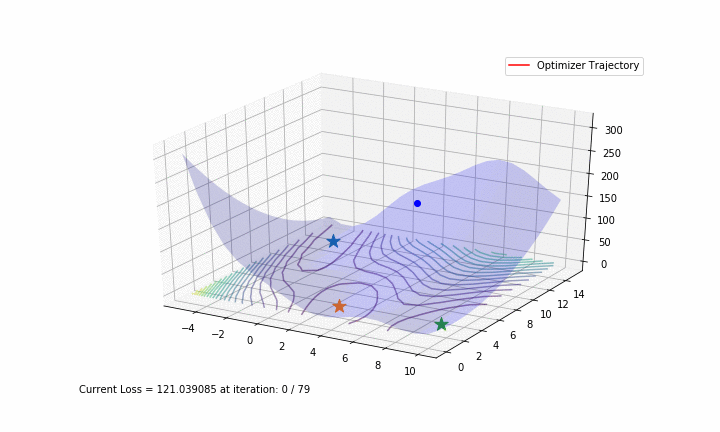
Trajectory of SGD on the stochastic Branin function. The blue function is the non-stochastic version, while the z-value is given by the (observed) stochastic function value.